Course Project, CS460, Fall 2021-22
On Federated Learning and Possible Improvements
Saswat Das
1811138 | saswat.das@niser.ac.in | School of Mathematical Sciences, NISER, HBNI
Suraj Ku. Patel
1811163 | suraj.kpatel@niser.ac.in | School of Physical Sciences, NISER, HBNI
Project Github Repository
1. Project Proposal (6 Sept 2021)
Introduction
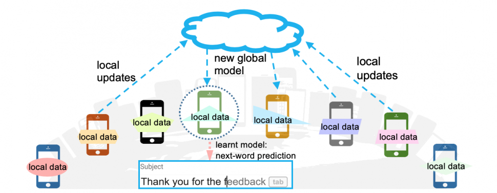
Federated learning (abbreviated as FL) refers to the practice of conducting machine learning based on several users' data by having each user, given an initial global model by a central server, locally train a model on their local devices, then communicate their locally trained model to the central server, following which each user's local model is aggregated at the central server with that of others, and used to update the global model.
This is in contrast to centralised learning, where the users' data would have been sent to the central server, and a model would have been trained on all that collected data in one central server.
Advantages?
Quite some!
- The user's personal data never leaves their local device, thus ensuring a healthy measure of privacy;
- Can possibly incorporate nuances of each user's local model by a suitable aggregation technique/algorithm to provide better, more nuanced learning.
Concerns/Areas of Possible Improvement
- Communication costs post local training and optimising number of communication rounds between each local device and the central server:
- Cost of computation due to local training on each device and effects on user experience during local training;
- Possible improvements in aggregation algorithms;
- Enhancement of privacy, and making sure no adversary can conclude from the (say, weights of the) local models an individual user's personal information or behaviour.
What we intend to do - a brief sketch
- Implement a Federated Learning algorithm (tentatively FederatedAveraging ) after locally training models using algorithms like SGD (as suggested) on generated datasets, or even implementing some neural network(s) if possible using popular datasets (viz. FEMNIST, Shakespeare, Sentiment140, CIFAR 10) if we are feeling bold. We can use TensorFlow and SherpaAI for this if possible/needed (no promises).
- Using the (local) learning algorithm as a baseline, we can compare the results of our FL based trained-and-aggregated model with centralised learning with the same algorithm, and some other popular algorithms.
- Suggest improvements to the paradigm just implemented in terms of
- The aggregating formula/algorithm;
- minimising rounds of communication and computational cost per local device; and/or
- enhancing privacy (viz. by adding differential privacy into the mix).
Then we will see how said tweaks work in terms of these metrics and report any observed improvements/changes (fingers crossed).
Midway Targets
- Successfully implement an FL model, and come up with some preliminary results;
- Suggest some tweaks and improvements to test out;
- If needed, present pertinent concepts from relevant literature.
Work Division
- Coding/Privacy based considerations - Joint task, will divide up coding of different components fluidly as needed.
- Data analysis and visualisation - Suraj
- Mathematics, formulae, proofs - Saswat
- Report writing and project website maintenance - Joint task
Expected Results
- Performance of FL based learning: almost as sound as if the learning was centralised, and maybe more nuanced.
- Either of these: Increased privacy, less communication rounds with the server, less/quicker local device computation, better aggregation.
Relevant Papers
- McMahan, H. B. et al. “Communication-Efficient Learning of Deep Networks from Decentralized Data.” AISTATS (2017).
- Konecný, Jakub et al. “Federated Learning: Strategies for Improving Communication Efficiency.” ArXiv abs/1610.05492 (2016): n. pag.
- Barroso, Nuria Rodríguez et al. “Federated Learning and Differential Privacy: Software tools analysis, the Sherpa.ai FL framework and methodological guidelines for preserving data privacy.” Inf. Fusion 64 (2020): 270-292.
Project Presentation Slides
2. Project Midway
Literature Review
Some of the most important papers we referred to are listed below.
- McMahan, H. Brendan et al. “Communication-Efficient Learning of Deep Networks from Decentralized Data.” AISTATS (2017).
- Konecný, Jakub et al. “Federated Learning: Strategies for Improving Communication Efficiency.” ArXiv abs/1610.05492 (2016).
- Wei, Kang et al. “Federated Learning With Differential Privacy: Algorithms and Performance Analysis.” IEEE Transactions on Information Forensics and Security 15 (2020): 3454-3469.
- Ji, Shaoxiong et al. “Dynamic Sampling and Selective Masking for Communication-Efficient Federated Learning.” ArXiv abs/2003.09603 (2020).
- McMahan et al
-
Introduces federated learning;
-
Addresses issues such as unbalanced volume of datapoints across all clients, limited communication capabilities of clients (via multiple rounds of communication), and the mass distributed nature of the clients, and the non-IID nature of data as an individual’s data is specific;
-
Introduces FedAvg ( \(w_{t+1}\gets\sum_{i=1}^K\frac{n_k}{n}w_{t+1}^k\) );
-
Talks about controlling parallelism of local computation and increased local computation by varying batch size for gradient descent (decreasing it increases amount/precision of computation, no. of rounds, and no. of clients queried per round (affects parallelism).
- Remarks:
- This provides us with a robust federated learning paradigm, but of course, as we shall soon see, this is a naive approach in terms of privacy, as there have supposedly been attacks in which adversaries have used weight updates in this scheme, say from a facial recognition application, to compromise the identities of users;
- Also this may seem pretty intuitive (and as we shall see, this works pretty well for SGD), it is sort of a simple arithmetic mean at the end of the day, and might be unable to capture some subtle nuances of the weight vectors received from clients, maybe some non linear aggregation formula could work better in certain contexts, and it is a good area to look into.
- The idea behind increasing parallelism by lowering the number of rounds of communication and increasing computation in between rounds locally by making the task at hand more precise (viz. by reducing batch size for gradient descent) is fairly intuitive, but is there a way to have clients with slower connections begin to upload their weight vectors for a certain (scheduled) round of communication prior to others with no such constraint? If so, how should rounds be scheduled?
- Wei et al
-
Introduces Gaussian noise w.r.t. a clipping parameter \(C\) to weight vector uploads, weights scaled w.r.t. \(C\) ;
-
Motivation: Naïvely uploaded weights carry the risk of being used by adversaries to compromise users;
-
Proposes uplink and optional downlink noise addition;
-
Takes fairly large values for the privacy budget;
-
Accuracy improves with no. of clients queried and rounds of communication;
-
Best accuracy when clients have (near) identical amounts of quality data;
-
Akin to central differential privacy, straightforward noise addition.
- Remarks:
- This is a fairly straightforward method of adding Gaussian noise (and ergo endow approximate differential privacy) into the weight uploads. But are there better ways of doing the same? We briefly considered implementing something similar using the exponential mechanism, and given how versatile it is, it could perhaps capture the nuances of the local training better, especially if you consider that out-of-bound (w.r.t. the clipping threshold) weight vectors are simply scaled down w.r.t. the clipping threshold (for good reason), can this be made more dynamic and inclusive of the factors and nuances in each client's dataset/model? It is an interesting thought.
- We also noticed that the authors do not mention a norm per se in the paper for the weight vectors while defining their algorithm (though there are some obvious choices, this was a bit unsettling).
- The authors use large values of the privacy budget (given the number of clients/the massively distributed nature of the client pool, this seems fair); can this be reduced while not having a major increase in error? Or with the minimum possible increase in the number of required clients to counteract any increase in noise?
- Konečný et al
-
Introduces methods to reduce the uplink communication costs by reducing the size of the updated model sent back by the client to the server.
-
Motivation: Poor bandwidth/expensive connections of a number of the participating devices (clients) leads to problems during the aggregation of data for FL.
-
Two methods for sending a smaller model are:
-
Structured updates, updates are from a restricted space and can be parametrized using a smaller number of variables. Algorithms: Low Rank and Random Mask.
-
Sketched updates, full model updates are learned but a compressed model update is sent to the server. Algorithms: Subsampling, Probabilistic quantization, and structured random rotations.
-
FedAvg is used for the experiments to decrease the number of rounds of communication required to train a good model.
-
Conclusions of the paper
-
Random mask performs significantly better than low rank, as the size of the updates is reduced.
-
Random masking gives higher accuracy as compared to sketched updates method but reaches moderate accuracy much slower.
-
Quantization algorithm alone is very unstable For a small number of quantization bits and smaller modes, and random rotation with quantization is more stable and has improved performance as compared to without rotation.
-
By increasing the number of rounds of training, the fraction of clients taken per round can be minimised without risking accuracy.
-
Introduced an important and practical tradeoff in the FL: one can select more clients in each round while having each of them communicate less, and obtain the same accuracy as using fewer clients, but having each of them communicate more.
- Note (The random mask's indices/low rank's encoding matrix can be elegantly encoded in a random seed, we haven't implemented it that way per se, though the idea is the same, but that is a fairly elegant manner of going about it, not to mention the significant advantage of terms of just having to remember a seed and not an array of indices/a matrix.)
- Extra: Ji et al
- Proposes dynamic sampling and selective mask;
- Dynamic sampling: In contrast to the usual way of sampling clients during each round of communication (i.e. static sampling), we define a decay constant, called \(\beta\), and if the initial sampling rate is \(C\) , then we choose \(\frac{C}{\exp(\beta t)}\) fraction of clients for round \(t\) (starting with \(t=0\) ) ;
- Selective mask: Instead of fully (uniformly) randomised selection of indices for a mask, choose the top \(k\) indices with the most significant updates to the initial model for each client;
- Selective mask consistently outperformed random mask in terms of accuracy and rate of convergence;
- Dynamic sampling gave accuracy comparable to static sampling, but at a significant loss in communication cost.
- Remarks:
- We have a few bones to pick here: while these work extremely well all things considered, would not it be better if dynamic sampling chose to sample a larger number of clients in response to an increase in observed error after a particular vis-a-vis previous rounds to help decrease the error for subsequent rounds? This could be a neat feature.
- Selective sampling chooses a specified number of the most significant (by magnitude) updates, and it definitely seems to be working really well, but we are concerned if in the process, i.e. by disregarding the others, we might be losing some important nuance in the process (i.e. this reasoning seems to be kind of reductionist and black-and-white). So can we instead choose mostly from among the top updates, and reserve a small proportion for those not in that club, so to speak? And if so, will this approach yield any advantages? Might as well try that out.
Techniques Used/Explored
-
For aggregation, we used FedAvg for the most vanilla FL implementation, and then added to it as necessary for the implementation of more sophisticated FL techniques;
-
The Gaussian Mechanism to provide \((\varepsilon,\delta)\) -differential privacy pre-upload from each device (Noising before Aggregation), as introduced by Wei et al.;
-
Static Sampling of clients for every round of training to reduce communication rounds per user;
-
Random Mask and Probabilistic Quantisation as described by Konečný et al;
-
Dynamic Sampling of clients to successively reduce the proportion of clients involved in successive rounds of communication to further save on rounds of communication and computational resources (as proposed by Ji et al);
-
Considering/considered using: Selective Mask (especially when working with larger weight vectors/matrices).
Experiments and Observations
We implemented FedAvg from scratch in Python, with a 0.25 static sampling rate, with anywhere between 3 to 5 (or more) rounds of calling for training from sampled (w.r.t. the uniform distribution) clients, with local training involving multiple linear regression implemented via Stochastic Gradient Descent on a synthetically generated dataset for about 500 clients, with static subsampling (contrast with dynamic subsampling).
The generated datasets, generated around a pre-chosen/generated "true weights vector" (we chose the dimension of these weight vectors to be 7) (e.g. \([1, 2, 4, 3, 5, 6, 1.2]\) ), are mostly IID as we focused more on implementing a model atop that.
As we are using regression here, we use, for a particular instance, average training/testing error per data point as a metric of a deployment’s accuracy, and simply measure the time taken by running it on Google Colab and compare them as a rough measure of how quick each is, and implement centralised learning to serve as a baseline for our exploration of these FL paradigms.
We then tried the above listed techniques, sometimes standalone or in conjunction with each other as follows.
- Centralised Learning (As a Baseline)
For centralised learning, we simply gathered and flattened the list of all local datasets into a cumulative list of all datapoints, and ran SGD on it for 100 epochs.
Time Taken \(\approx 268-270\) seconds.
Average Training Error for Centralised Learning on SGD \(\approx 3.2472\times 10^{-29}\).
Average Testing Error for Centralised Learning on SGD \(\approx 3.2154 \times 10^{-29}\).
- Vanilla
FederatedAveraging/FedAvg
We then ran vanilla FedAvg with static sampling of clients at a rate of 0.25 of the client population per round of training on the above mentioned local datasets, with 100 epochs per round of local training. Number of rounds, \(T=5\) .
Time taken \(\approx 362\) seconds.
Average Training Error for Vanilla FedAvg on SGD \(\approx 2.5331\times 10^{-18}\) .
Average Testing Error for Vanilla FedAvg on SGD \(\approx 2.6021\times 10^{-18}\) .
- Noising before Aggregation (From Wei et al)
Adds Gaussian noise to appropriately clipped weights from each user. Motivation: To stop attacks involving reconstruction of raw data/private information from naïve uploading of weight vectors/matrices. Optionally adds downlink DP, but we felt it was unnecessary.
We ran FedAvg with static sampling of clients at a rate of 0.25 per round of training, clipping the locally generated weight vectors to gain bounds (defining upper bound of the norm of a weight vector as \(C =1.01\times\max(w_i)\) , where \(w -\) weight vector, for the sake of computing the sensitivity of queries for the weight vectors, then adding Gaussian noise calibrated to \(C,\varepsilon,\delta\) to each weight ( \(\varepsilon=70,\delta=0.1\) ) with 100 epochs per round of local training. Number of rounds, \(T=5\) .
Time taken \(\approx 349\) seconds (which makes it about as fast as vanilla FedAvg).
Average Training Error for NbA FedAvg on SGD \(\approx 7.2562\times 10^{-7}\) .
Average Testing Error for NbA FedAvg on SGD \(\approx 6.6740\times10^{-7}\) .
- NbAFL with Random Mask
We use the same setup as for the above NbAFL implementation, but with a layer of uniformly chosen random masks, excluding \(\approx s=0.25\) of the weights, prior to uploading by a client. Seems to consistently outperform base NbAFL in terms of accuracy, also reduces communication overhead!
Time taken \(\approx 356\) seconds.
Average Training Error \(\approx 0.006601\).
Average Testing Error \(\approx 0.007577\).
- NbAFL with Probabilistic Binarisation
We again use the same setup and parameters as our vanilla NbAFL implementation, but with probabilistic binarisation implemented atop it.
Time taken \(\approx 356\) seconds.
Average Training Error \(\approx 0.021241\) .
Average Testing Error \(\approx 0.019635\)
- NbAFL with Dynamic Sampling
We again adopt the same setup as that for our vanilla NbAFL implementation, but instead of static sampling of clients, we sample clients with an initial rate of \(0.25\) , which decays by a factor of \(\frac 1{\exp(\beta t)}\) , where \(t =\) number of rounds elapsed. We take \(\beta=0.05\) .
Time taken \(\approx 334\) seconds.
(Saves on time and no. of communication rounds!)
Average Training Error \(\approx 0.010684\) .
Average Testing Error \(\approx 0.010908\) .
The following table summarises the parameters used for and the results of our experiments (to be fair, we had to fiddle with a fair of different values for parameters and variations in algorithms to fix these for now)
Local Learning Rate, \(\alpha = 0.01\) ; No. of local iterations for SGD \(=100\) , No. of clients \(=500\)
| Centralised SGD |
- |
- |
- |
- |
\(3.2472\times 10^{-29}\) |
\(3.2154 \times 10^{-29}\) |
268 - 270 |
- |
Vanilla FedAvg |
5 |
0.25 |
- |
- |
\(2.5331\times 10^{-18}\) |
\(2.6021\times 10^{-18}\) |
362 |
- |
| NbAFL |
5 |
0.25 |
70 |
0.01 |
\(7.2562\times 10^{-7}\) |
\(6.6740\times10^{-7}\) |
349 |
- |
| NbAFL w/ Random Mask |
5 |
0.25 |
70 |
0.01 |
0.006601 |
0.007577 |
356 |
\(s=0.25\) |
| NbAFL w/ Prob. Bin. |
5 |
0.25 |
70 |
0.01 |
0.021241 |
0.019635 |
356 |
- |
| NbAFL w/ Dyn. Samp. |
5 |
0.25 |
70 |
0.01 |
0.010684 |
0.010908 |
334 |
\(\beta=0.05\) |
Note that the errors happen to be quite small compared to the weight vectors' magnitude, with a maximum being in the neighbourhood of 1% error to "true" weight vector (norm/coordinates) ratio, roughly.
Suggested Tweaks and Possible Improvements to Try Out to Extend the Baselines
-
Silo-ing users with similar characteristics and running a separate FL paradigm within these silos;
-
Applications to dapps (decentralised applications) on P2P networks (given that uploaded weight vectors are more or less public and aggregation does not take much time);
-
Trying other mechanisms (viz. exponential) out on NbAFL for possible improvement, or explore locally differentially private techniques instead (some baseline work on this exists);
-
Trying Selective Mask from out, and slightly diffusing the choice from the top \(k\) updates to some of the lower updates;
-
Making dynamic sample more dynamic and efficient by calibrating decay w.r.t. error per round of communication (more error \(\implies\) less decay;
-
Exploring mutual benefits of probabilistic quantisation and noise addition, calibrating no. of quanta to the magnitude of the noise;
-
Looking at tweaks to FedAvg in certain contexts;
- Think of how to further unlink clients from their uploaded weights (perhaps mixes will help);
-
Anything else that strikes our minds.
We may tentatively try implementing the above FL models for more complex local training algorithms (viz. ConvNets using FEMNIST), but this is secondary/optional.
Here is the link to the .ipynb file containing the midway version of our code.
Some Midway References
- H. B. McMahan, E. Moore, D. Ramage, and B. A. y Arcas,
“Communication-efficient learning of deep networks from
decentralized data,”, 2016.
- K. Wei, J. Li, M. Ding, C. Ma, H. H. Yang, F. Farokhi, S. Jin,
T. Q. S. Quek, and H. V. Poor, “Federated learning with differential
privacy: Algorithms and performance analysis,” IEEE Transactions on
Information Forensics and Security, 2020.
- J. Konecny, H. B. McMahan, F. X. Yu, P. Richt ́arik, A. T. Suresh,
and D. Bacon, “Federated learning: Strategies for improving
communication efficiency,” CoRR, vol. abs/1610.05492, 2016.
- S. Ji, W. Jiang, A. Walid, and X. Li, “Dynamic sampling and
selective masking for communication-efficient federated learning,”
CoRR, vol. abs/2003.09603, 2020.
Midway Presentation Slides
(Kindly Exclude The Title and Bibliography Slides from the Slide Count)
3. Final Project Presentation/Extension of Baselines
Since the midway, we did a number of things, the most notable of which are as follows.
-
Created a federated learning code framework from scratch to transfer our work from one that employs local learning via linear regression on a randomly generated dataset to one that employs DNNs (implemented on Tensorflow) to classify digits in MNIST (randomly shuffled and distributed across clients).
-
Tried out various approaches and tweaks to some existing paradigms/models.
-
Designed "Adaptive Sampling" an improvement to Dynamic Sampling, with penalisation of the sampling decay coefficient for increase in errors.
-
Designed a fully decentralised P2P approach to FL (in contrast to the recent P2P models proposed that involve a level of temporary centralisation).
-
Designed an approach involving clustering (of clients) in silos and simultaneously training a silo-specific model and a general model via FL.
Specifications of our new framework
-
MNIST (training data shuffled and distributed unequally at random among 100 clients)
- Local Training:
-
Via a DNN, defined and compiled with Tensorflow.
-
Input Layer: Flatten Layer.
-
Hidden Layers: 32 units and 512 units* (later ditched for speed) with ReLU activation.
-
Dropout Layer* (rate = 0.2): Before the \(2^\text{nd}\) Hidden Layer (later ditched)
-
Output Layer: 10 units with Softmax activation.
-
Batch Normalisation: Before every hidden and output layer
In a nutshell, due to time and computing power constraints, we ended up using a DNN with a flatten layer, a hidden layer with 32 units with ReLU activation, followed by an output layer with 10 units with softmax activation, not to mention the batch normalisation layers before the hidden and output layer. As we shall soon see, we found that this was sufficient to give a high degree of accuracy on MNIST.
- Federated Averaging was implemented similarly as for our older framework, as per the original paper on Federated Averaging by McMahan et al.
A salient feature of our framework is that it is flexible enough to be used for any Tensorflow based neural network (at least ones that are created using keras.sequential) and for any dataset that is fed into such an NN.
N.B. For testing, we initialised the same server model (i.e. we started training with a weight vector that was common for every run, for example, a weight vector with all 0s for each "coordinate" in the vector) for each run of each model, for a fair comparison.
Given the conception of the new code framework with the DNN on MNIST, we re-ran some of the relevant baselines using it, and we got the following results. Please note that the provided figures/graphs are representative, as in they are just a few from the many runs of each model/algorithm.
Centralised Learning
Which simply is training the DNN using all of the MNIST training data in one place, and precisely what any federated learning algorithm should aspire to match, or at least approach, in terms of accuracy.
Test Accuracy: 96.52% (Pretty nice!)
Which, as mentioned earlier, is simply an implementation of McMahan et al's model with aggregation via FederatedAvg. Note that here in each round of communication, a fixed proportion of the total number of clients are asked for local updates, which in the language of client sampling is called static sampling.
Number of Communication Rounds: 50
Test Accuracy: 94.21% (Not bad at all!)
FedAveraging with Dynamic Sampling
For a proper recaptitulation of what Dynamic Sampling does, refer to our prior discussion regarding Ji et al in the Midway section. But in a nutshell, what it does is reduce the number of clients sampled per round w.r.t. a decay coefficient \(\beta\) and the initial client sampling rate (i.e. by multiplying \(\frac 1{\exp(-\beta t)}\) to the initial sampling rate).
Decay Coeff. \(\beta\) : 0.05
Initial Sampling Rate : 0.25
Test Accuracy: 93.7%
Number of Rounds: 50
Note that dynamic sampling decreases the number of clients per round independent of the change of accuracy per round.
The problem? This can slow down convergence and error rectification, or even occasionally and briefly lead to consecutive increases in error because aggregation of several client weights leads to a good aggregate weights estimate, but instead, the number of clients is continually decreasing here with the naive approach that decreasing the number of clients per round would decrease the volume of communication. Okay, that is true, but especially in a short term manner. In the long term, slow error rectification will lead to the model requiring a larger number of rounds of communication, which incurs both a time cost and communication cost in that way. But we can see that the thinking behind this paradigm is not without merit, we got a really good accuracy for substantially less clients' involvement vis-a-vis the vanilla case. But can we couple the reduction of the number of clients with faster convergence in a way that we are fine having the initial decay coefficient (which is positively correlated to how fast the decay occurs) as long as the error does not increase beyond a previously attained error value, at which point we would want to slow down the decay and make sure to involve more clients than in the last round to mitigate the amount of error and bring the amount of accuracy eventually to the highest previously attained accuracy beyond which it fell off. This is precisely the motivation behind us introducing adaptive sampling.
More clients involved \(\implies\) Better averaging \(\implies\) Less error.
I. Adaptive Sampling
That is, we keep successively penalising the decay coefficient for any fall in accuracy, while retaining the previous index, so as to increase the number of clients for the next round and slow the decay in the sampling rate down, and restore the decay coefficient when accuracy reaches the previous high.
The pseudocode for adaptive sampling is as follows.
Note : \(n_i\) is the number of datapoints possessed by the client corresponding to \(\Omega_t^i\) , and \(n\) is the total of all \(n_i\) ’s for each \(\Omega_t^i\in L\) .
Also, note that \((\gamma)\) is just a parameter we introduced in case we needed to tune the penalisation of the decay coefficient, and we kept it equal to 1 to start off with, and as it turned out, that worked just fine, so we kept it at 1.
We again ran several rounds of experiments for adaptive sampling and some representative results, with similar parameters as for the previous representative run for dynamic sampling, are as follows:
Initial Decay Coeff. \(\beta\) : 0.05
Initial Sampling Rate : 0.25
Gamma \((\gamma)\) : 1
Test Accuracy: 94.16%
Rounds of Communication: 20
(It would have risen as accuracy fell in the last step; it had an accuracy of 94.59% after round 19, but since we only specified 20 rounds of communication, it stalled at that.)
What immediately jumps out at us upon viewing this graph is that 1. it seems to lead to smoother convergence, sans any of the jaggedness as for dynamic sampling; and 2. it leads to convergence within lesser rounds of communication, albeit with marginally more clients per round on average being involved than dynamic sampling (owing to the penalisation of the decay coefficient at times along with stalling of the counter variable whenever accuracy drops), and knowing/assuming that the server calls on clients for communication round wise and clients in each round upload their local weights nearly simultaneously, lesser number of rounds implies lesser time taken for this entire exercise of federated learning.
II. Fully Decentralised P2P FL Learning:
In federated learning, the server aggregates the weight vector of the devices to make a new model, which implies a significant degree of centralisation, which in turn creates a single entity for an adversary to attack or track communications to; alternatively, sending weights to a central server might not be desirable in certain contexts for the sake of privacy.
In addition, traditional federated learning does not address its implementation for P2P networks, which has much potential given the advent of decentralisation to the extent that we see nowadays, and that of smart contracts and decentralised apps (dapps). Naturally, this has been a recent field of inquiry as far as federated learning is concerned.
So, we decided to formulate a model for peer-to-peer learning where local training is done for all the peers involved in a round of training, and then after exchanging local weights among themselves, each device independently performs aggregation via FedAveraging (which in itself is not exactly an expensive task), and can compare the newly aggregated model with their existing ones to see what works best for them, and as a secondary consequence, guard against injection of illicit values by any malicious peer(s) (and we also gave quite some thought on how to nullify/penalise the malicious peer's influence or even remove them entirely in such an event).
Baselines for P2P Learning
To reiterate, federated learning in the context of P2P networks (i.e. sans a server) is a nascent field of study.
Some of the earliest models like BrainTorrent (2019), and that by Behera et al (JPMorgan Chase & Co., 2021) involve taking (i.e. randomly choosing/electing) a temporary "leader" peer node to act in the capacity of the server, thus inducing a level of centralization, and the peers having to accept the leader’s aggregation in good faith.
Others like FedP2P (2021) involve a model wherein a central server organizes clients into a P2P network after some bootstrapping is done at the server-end, and are not suitable for fully decentralized P2P networks.
Then there are models like IPLS (2021) involve a client acting as a central "leader/server" that assigns tasks to its peers, which resembles task delegation more than imploring devices to work on their own data and their own data only.
All of the serverless models we have come across involve making a peer a "temporary leader/server", and thus have a level of centralization, which brings privacy risks along with it. We aim to remove this aspect to obtain a completely decentralized FL paradigm for P2P networks.
Description of the Algorithm:
-
A dapp or smart contract specifies an initial random model for all the devices in a round of communication/training.
-
A device/peer may send a call for updates to all its peers, periodically or of its own volition.
-
If a good enough proportion of peers agree, then they initialize with a common initial model (specified within the contract initially, else the last shared global model), and train local models. The last 2-3 "accepted" global models for a peer, if any, are stored locally.
-
Each device calls for a number of those locally trained weights from a significant proportion (or all) of its peers and aggregates it.
-
If the model performs better than its existing model, it keeps it (updates the local instance of dapp/smart contract accordingly), else ditches it.
Peers query for how many models ditched the new global model, if a majority do, then initialize the next round of training with the last viable one. (Defends the system against erroneous value injection.)
In our experiments for our P2P federated learning mode, we simulated 100 peers/clients on the aforementioned framework on DNNs/MNIST, with a 0.25 client sampling rate. (Though, practically speaking, all this does is explore the case when 0.25 peers decide to participate in a round of training per round, though perhaps in a real life implementation, it may very well go beyond that, as peers shall seek to maximise the number of them that participate in a given round. 25% of clients chosen at random seemed to be a pretty good conservative estimate to us.)
Another caveat: we assume the absence of a malicious peer here, though should one be there, it cannot cause any damage due to each peer choosing the best of the current and the new model, and the only way the adversarial peer can "succeed" is by ensuring that the new model post-aggregation is better than the current model(s) already implemented on the devices, which is not exactly a win for any malicious peer intent on derailing the learning process, and if an aggregated model happens to be way off the rails due to adversarial interference and rejected by a majority of the peers, it shall be rejected entirely and the most recent accepted common aggregated model shall be agreed upon to continue training from the next round onwards. (Note that this shall work especially well on P2P networks with defences against Sybil attacks.)
Results of Decentralised P2P Fed Learning
| Round 1 (Initial) |
93.79% |
93.84% |
92.67% |
93.49% |
| Round 2 |
94.25% |
94.31% |
92.77% |
94.02% |
| Round 3 |
94.75% |
94.82% |
93.97% |
94.48% |
| Round 4 |
94.71% |
94.99% |
93.80% |
94.62% |
| Round 5 |
94.87% |
94.98% |
94.38% |
94.76% |
| Round 6 |
94.97% |
95.09% |
94.25% |
94.85% |
| Round 7 |
94.92% |
95.14% |
93.80% |
94.90% |
And here's a supporting graph to better visualise these values. Note that the max, min and mean accuracies in the sample refer to those within the subcollection of peers that have participated in a given round. Of interest are the trends of shared global model accuracy (which approaches the baseline vanilla FedAvg accuracy) and the mean cluster/sample accuracy.
 So what do we see here? That there seems to be an overall upward trend across the board for all these different statistics, which seems to perfectly suit the end goal of training using federated learning without a server. Also, we can see that even if a peer had not participated in training for a few rounds when it does go for training, it attains accuracy comparable to its other peers in the sample with accuracy (most probably) higher than that for the preceding rounds. (This is not very surprising of course, but it is a desirable property to possess.)
Some Concerns
-
A large proportion of peers must ideally agree for a round of communication, and there might be rounds wherein not a lot of peers would agree. Form of round scheduling might help in this regard, perhaps.
-
Outliers may cause problems. (This is true for vanilla FedAvg anyway, so is not an exclusive concern to this model.)
-
Inter-peer bandwidth could be a bottleneck in P2P networks, so we would do well to reduce communication size somehow (and as mentioned earlier, this can be achieved by the use of a number of well known communication overhead reducing techniques).
-
What about a malicious peer reporting incorrect weights? That’s solved; inaccurate models thus aggregated are rejected by peers, as emphasised earlier. Ideally, one would also want to find a way to either isolate, reduce the influence of or entirely remove the malicious peer. (viz. by a multiplicative weights approach, a peer could reduce a weight corresponding to a peer's reputation whenever it ends up with a less accurate model than the one it already has, and as a result, either decrease the weight accorded to the weight vectors of peers in the subcollection of peers in that communication round or call these peers less often; this is an open line of inquiry at the moment.)
Serving Suggestions (a.k.a. Possible Augmentations to consider while implementing practically)
-
For the security of communication, we can use something like hybrid encryption to encrypt weight vectors in transit (to protect against eavesdropping adversaries, including non-peers).
-
For increasing privacy, differentially private noise can be added.
III. Subclustering of Clients w.r.t. their Local Updates and Creation of Specific Models for Minority Clusters
In general FL techniques create a common model useful for the majority of devices, suffices for most purposes, but in this process, any minor clusters of devices having different data (and ergo producing different weight vectors post local training) than most may benefit from getting more specific models appropriate for their data in certain contexts.
Algorithm:
-
We start with a regular FL (viz. Vanilla FedAvg) approach to training an FL model.
-
Local models of all the devices are clustered (using DB-SCAN) based on their weight vectors.
-
All the devices having the same cluster-id are extracted, and federated averaging is done only for those devices (in a P2P manner). This process is repeated until a model is formed for every cluster.
-
These weights are returned to the server to provide a model for devices having a different and smaller class of dataset. Devices may opt to use the general model or the specific model, if any.
Note about Baselines and an Augmentation we Made
Some background on our (admittedly unorthodox) method of creating this model: one of us had actually conceived this while brainstorming all that we could get up to whilst cooking up and testing new models, and we implemented it to see whether it runs properly on simulated data (created in a way so that there are indeed minority classes devices that have similar data but are different in comparison to most other devices). Post that, we proceeded to look at models that might have a similar approach.
Most baseline algorithms that we saw during our literature review suggested that most of the work that resembled this vein of thought was implemented by clustering devices based on their data itself in some fashion. We on the other hand chose to cluster devices based on the similarity between the local weights produced after local training during each round. (An honourable mention of such a baseline approach that the instructor pointed out would be FLaPS by Paul et al which one of the authors had gone through in the past but did not recall when the other author actually came up with this approach.)
Unfortunately, at a much later stage, it seemed that there was indeed a similar work (with respect to an older version of our model) done by researchers at Keele University, UK (Briggs et al.) with minor differences from our initial model.
So we went ahead and explored adding a P2P component to intra-silo (i.e. within each minority class/cluster) training of specific models, which would endow an additional benefit in terms of each silo getting to keep their weights private; now this would not matter when the server is aware of the clustering pattern as it can easily compute the specific models, but let's say that a group of clients (say they belong to the same organisation/lab) opt to define (among themselves only, assuming they are all connected as peers) a cluster of their own, regardless of the cluster they have been accorded in that round, then given that the server is not made aware of that custom-defined silo/cluster, the specific model would stay private to the members of the cluster.
In short, this augmentation allows clients flexibility to define their own clusters, even if that mightt not give them optimal accuracy.
Experimental Results (with P2P Intra Silo Learning Implemented)
Total number of devices: 125
Number of federated learning rounds(T): 10
Client Sampling Rate (per round): 0.25
Results of Subclustered FL
| |
No. of Devices |
For Global Model |
For Cluster Specific Models |
| Majority Cluster |
110 |
\(\approx\)0.00203 |
\(\approx\) 6.71926 \(\times 10^{-15}\) |
| Minority Cluster 1 |
8 |
\(\approx\)0.15474 |
\(\approx\) 6.30220 \(\times 10^{-13}\) |
| Minority Cluster 2 |
7 |
\(\approx\)0.12130 |
\(\approx\) 6.59985 \(\times 10^{-16}\) |
This goes on to show that for non-IID data or situations with clients that have different data could do well to utilise subclustering like this to obtain well-performing specific models.
We have only conducted testing for the clusters obtained via DB SCAN on the weight vectors using the older framework (as we ran into time constraints and issues involving implementing DB SCAN on the (even flattened) weights of NNs produced using Keras.
Note that we focused more on simulating these clusters in essence in that older framework, and the code would look more general in real-life use cases (in fact the not-successful code on the DNN/MNIST framework should be general in the abovementioned sense and closer to possible real-life implementations of this.)
(Accuracy on custom-defined clusters has not been tested for given time constraints and that it is an option to be opted for at the clients' discretion and risk. Though given the errors on the global model be, one can expect errors to that tune or even less.)
Possible Future Improvement(s)
Code Links (for the Final Presentation's Material/Models):
Final Presentation Slides
(Kindly Exclude The Title and Bibliography Slides from the Slide Count)
Some Additional References for the Final Presentation
(In addition to the ones already mentioned in prior presentations.)
- Monik Raj Behera et al. Federated Learning using Peer-to-peer Network for Decentralized Orchestration of Model Weights. Mar.
2021.
- Li Chou et al. “Efficient and Less Centralized Federated Learning”.
In: CoRR abs/2106.06627 (2021).
- Abhijit Guha Roy et al. “BrainTorrent: A Peer-to-Peer Environment
for Decentralized Federated Learning”. In: CoRR abs/1905.06731
(2019).
- Shaoxiong Ji et al. “Dynamic Sampling and Selective Masking for
Communication-Efficient Federated Learning”. In: CoRR
abs/2003.09603 (2020).
- Christodoulos Pappas et al. “IPLS : A Framework for Decentralized
Federated Learning”. In: CoRR abs/2101.01901 (2021).
- Briggs, C., Fan, Z., & András, P. (2020). Federated learning with hierarchical clustering of local updates to improve training on non-IID data. 2020 International Joint Conference on Neural Networks (IJCNN), 1-9.
- Sattler, F., Müller, K., & Samek, W. (2021). Clustered Federated Learning: Model-Agnostic Distributed Multitask Optimization Under Privacy Constraints. IEEE Transactions on Neural Networks and Learning Systems, 32, 3710-3722.
- Kim, Y., Håkim, E.A., Haraldson, J., Eriksson, H., Silva, J.M., & Fischione, C. (2021). Dynamic Clustering in Federated Learning. ICC 2021 - IEEE International Conference on Communications, 1-6.
We would like to take a moment to express our gratitude to Dr. Subhankar Mishra, not to gain any additional brownie points but to give credit where it is due, for urging us to consider working on federated learning for this project in the first place, which made all of this possible, and for his encouragement and guidance in this respect.
And also to the copious amounts of caffeine that fueled this project.


